Note that all results are not yet been published online as some of them take a lot of time to compute (especially renderings).

Individual results

A lot of information can be retrieved from each surface. Individual results are found in three different pages detailed below.

The header of each page contains global information about the data and ways to select a new surface:

The order used to go through the data. You can choose to sort the surfaces according to their index (sorted by name in each dataset) or to each numerical value (error E, prediction P, RMSE between renderings, or different statistical features).
Its name. The dropdown can be used to select an other surface, as well as the text input just aside. You can also go through all surfaces by pressing keys left < or right >.
Its rank in the current chosen order.
Its error E, its prediction P, and its RMSE between renderings (with uncorrelated or correlated GAF G) and their corresponding ranking among the whole dataset.

Overview

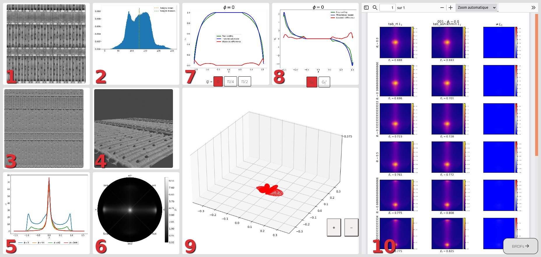
Each surface has a dedicated page that gives different details on its data. The details include:

Greyscale map of the height field.
Histogram of heights (from height field).
Shaded image of height field (seen from top).
Shaded image of height field (seen from aside).
Normal Distribution Function, sliced along four different Φ angles.
Normal Distribution Function, as projected on the tangent plane.
Masking term G₁ from the ray casting and theoretical models for three different Φ angles.
First and second derivatives of the masking term G₁ from the ray casting and theoretical models and their differences (displayed with the same Φ as selected for G₁). It is useful to see that the theoretical model cannot well reproduce inflection points (when G₁'' changes sign).
Absolute difference for each computed direction between the ray casting and theoretical G₁, and their differences. For each surface, plots are drawn at the same scale, but you can zoom in/out with the + and - buttons to modify the scale.
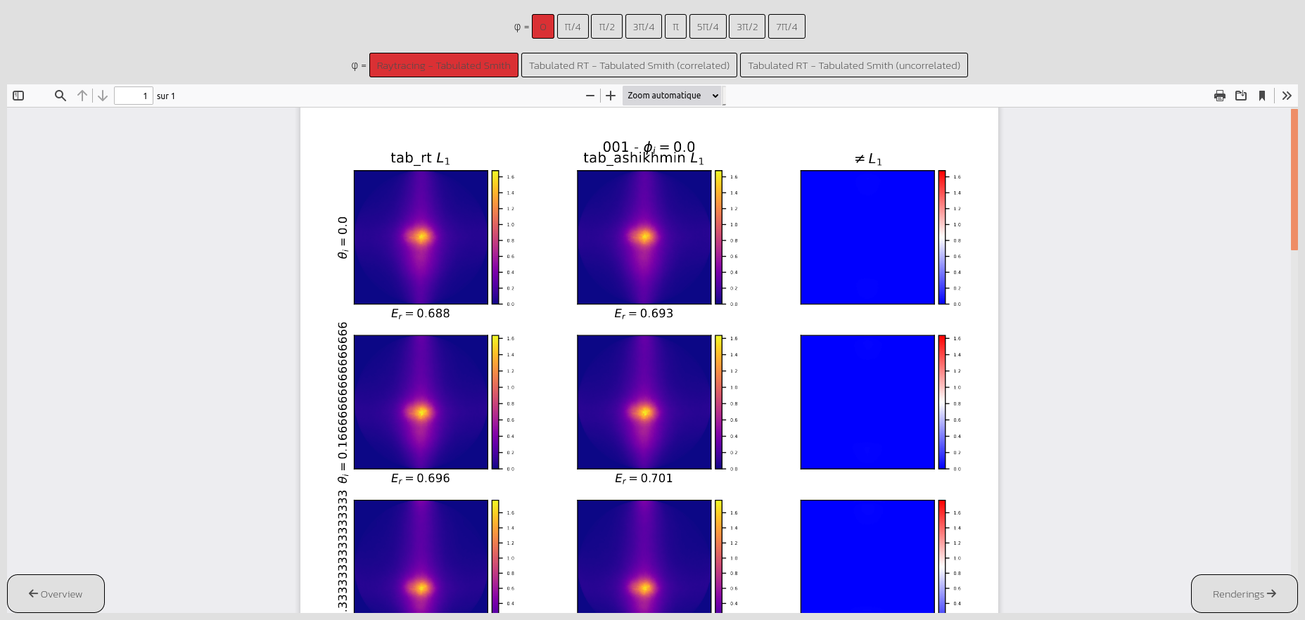
The BRDF computed with the ray casting masking term (tab_rt) and the theoretical masking term (tab_ashikhmin). Their differences are shown in the third column. Φ is fixed as chosen for the G₁ graph.

BRDFs

For more details on a given BRDF, one can choose between eight Φ.

Renderings

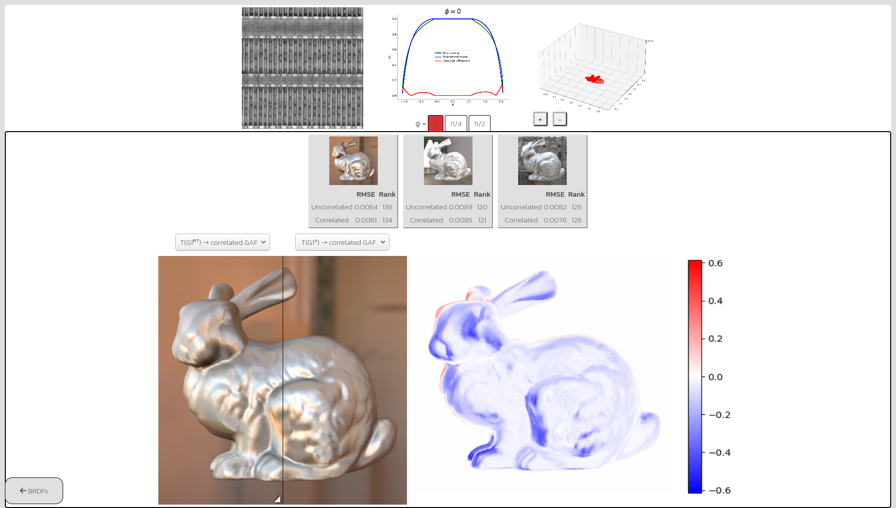
To compare renderings of materials of a given surface with both ray casting and theoretical G₁, this page gives the two images loaded at the same location, but with a slider to show one image vs. the other on the left/right of the slider. An image with a color map of the differences appears to the right. They are available for three different incident illumination maps, as shown above, with their rankings and values in RMSE. The greyscale map of the height field, its different models at slices of Φ, and absolute differences are also provided on the top of the page.

All results

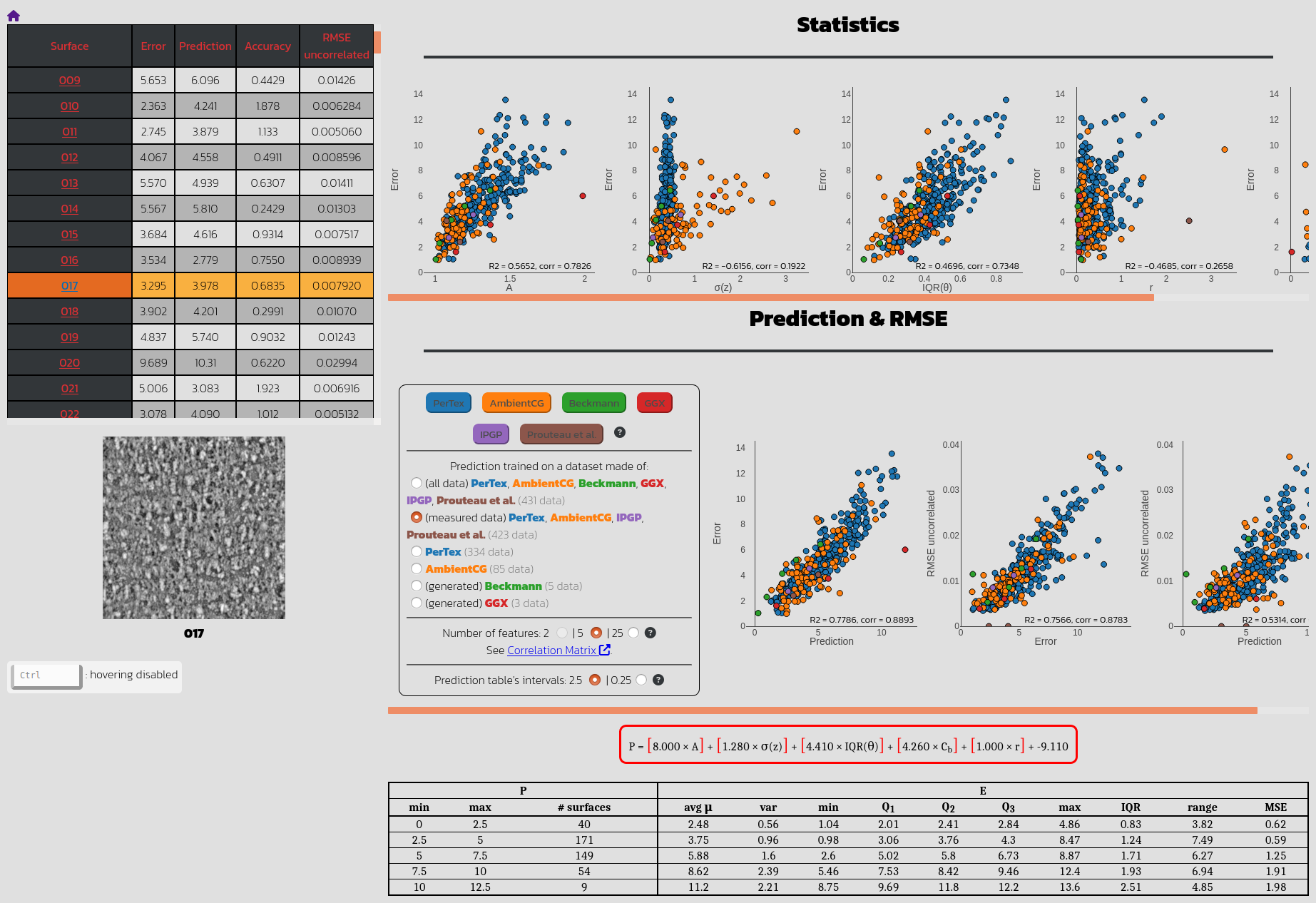
This page is useful to see all the results in one place. It is interactive and allows the user to hover over the data to directly visualise corresponding height fields. Below is a more detailed guide.

Settings

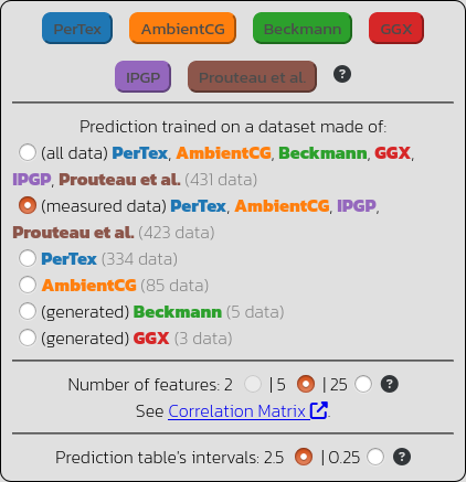
Different datasets have been used in our analysis.

PerTex: 334 heightfields measured with the same setting (embossed textures, blown vinyl, woven wall coverings, carpets and rugs, window blinds, soft furnishing fabrics, building materials, and product packaging);
AmbientCG: 85 heightfields measured with different settings (soils, rocks, floorings, and various materials);
IPGP: 2 heightfields measured with a drone (volcanic terrains);
Prouteau et al.: 2 measured heightfields (road pavement);
Beckmann: 5 generated heightfields from Beckmann isotropic distributions (α ∈ {0.1, 0.25, 0.5, 0.7, 1.0})
GGX: 3 generated heightfields from GGX isotropic distributions (α ∈ {0.25, 0.5, 1.0}).

Click on each button to show or hide the corresponding dataset in the graphs.

"Prediction trained on a dataset made of": choose which prediction model is shown depending on the data it was trained on. By default, it is selected to show a training on all measured data that we have (423) as in the paper.

"Number of features": predictive model presented in the paper is a linear combination of 5 features. But we can use 25 features to have a more precise prediction.

"Prediction table's intervals": choose the precision of the prediction table, i.e. the range of each interval is of 2.5 or 0.25.

Graphs

Push the key Ctrl to enable (green)/disable (grey) the hovering interaction with the data. It allows to display corresponding height field in the dedicated area but can require heavy loading ressources.

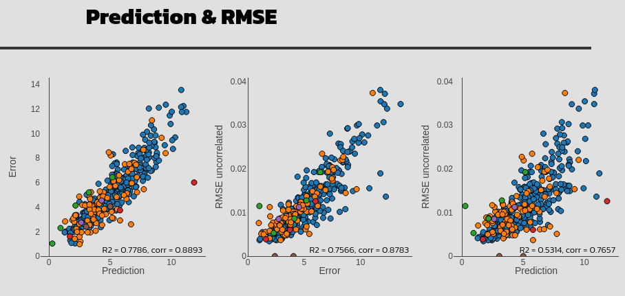
For each feature used for the predictive model, the error E is plotted against this feature. Plots are ranged by increasing order of importance in the linear combination.
If hovering is enabled (toggle by pressing Ctrl), hover your pointer on the points to show corresponding heightfield in the bottom left corner of the webpage. Click on a point to open a new tab redirecting to the analysis of this specific surface.

First graph shows the error E against the predictive resulting model P.
Second graph shows the average RMSE between three renderings with different environment map against the error E.
Third graph show the average RMSE against the prediction P.

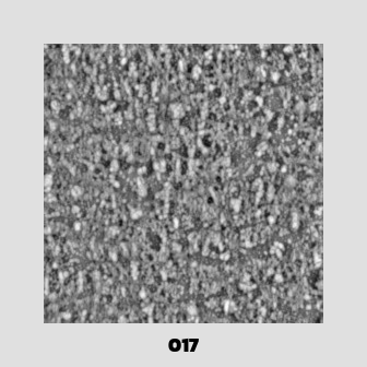
Height fields are displayed in the bottom left corner of the web page when hovering is enabled (toggle by pressing Ctrl). Click on the surface to open a new tab with the image at a higher quality.

Prediction table

Each row of this table shows the error statistics for a given prediction's interval. For a prediction between P_min and P_max, we can see how many surfaces lies in this interval and what their error is (described by the average, the variance, the range, the quartiles and the MSE).

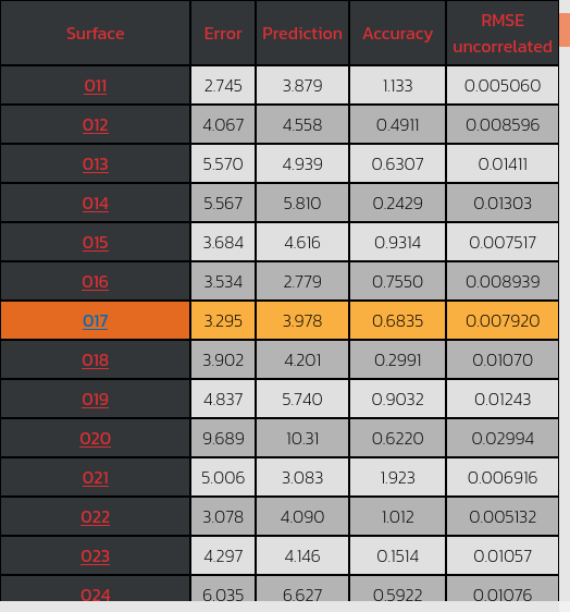
Sortable table

This table can be used to sort elements in increasing or decreasing columns (surfaces names, error E, prediction P and renderings RMSE). Hover your pointer on a row to display the corresponding height field beneath the table. Click on a surface name to open a new tab redirecting to the overview of this specific surface.